Understanding BIG O Calculations

Big O notation is a way to describe how the algorithm grow as the input size increases. Two things it considers:

Runtime
Space

1. Basic Idea

What It Measures:
Big O notation focuses on the worst-case scenario of an algorithm’s performance. It tells you how the running time (or space) increases as the size of the input grows.
- Guarantee of Performance:
  Worst-case analysis provides a guarantee that the algorithm won't perform worse than a certain bound, regardless of the input.
- Adversarial Inputs:
  In interviews, interviewers often assume inputs that force the algorithm to perform at its worst, so understanding the worst-case behavior is crucial.
- Comparing Algorithms:
  Worst-case complexity gives a clear basis for comparing different algorithms, ensuring that you choose one that performs reliably under all conditions.
Ignoring Constants:
It abstracts away constants and less significant terms. For instance, if an algorithm takes 3n + 5 steps, it’s considered O(n) because, for large n, the constant 5 and multiplier 3 become negligible compared to n.

2. Common Time Complexities

In order of least dominating term O(1) to most dominating term (the one that grows the fastest)

O(1) – Constant Time:
The runtime does not change with the size of the input.
- Example: Accessing an element in a list by its index.

O(log n) – Logarithmic Time:
The runtime increases slowly as the input size increases.
- Example: Binary search in a sorted list.

O(n) – Linear Time:
The runtime increases linearly with the input size.
- Example: Iterating through all elements of an array to find a specific value.

O(n log n):
Often seen in efficient sorting algorithms like mergesort or heapsort.
- Example: Sort the list in O(n), then use a Binary search in a sorted list O(logn).

O(n²) – Quadratic Time:
The runtime increases quadratically as the input size increases.
- Example: Using two nested loops to compare all pairs in an array.

3. Understanding Through Examples

Constant Time – O(1)

def get_first_element(lst):
    return lst[0]

Regardless of list size, only one operation is performed.

Linear Time – O(n)

def find_max(lst):
    max_val = lst[0]
    for num in lst:
        if num > max_val:
            max_val = num
    return max_val

In the find_max function, every element is inspected once, so the time grows linearly with the list size.

Quadratic Time – O(n²)

def print_all_pairs(lst):
    for i in range(len(lst)):
        for j in range(len(lst)):
            print(lst[i], lst[j])

Here, for each element, you’re iterating over the entire list, leading to a quadratic number of comparisons.

4. Why Big O Matters

Performance Insight:
Understanding Big O helps you predict how your solution will scale.
- O(n) solution will generally perform better than an O(n²) solution as the input size increases.
Algorithm Choice:
It allows you to compare different algorithms and select the most efficient one for your needs.
- Discussing Big O can show your understanding of algorithm efficiency.

5. Space Complexity

Just as you can analyze time complexity, Big O also helps you understand how much memory an algorithm requires relative to the input size.

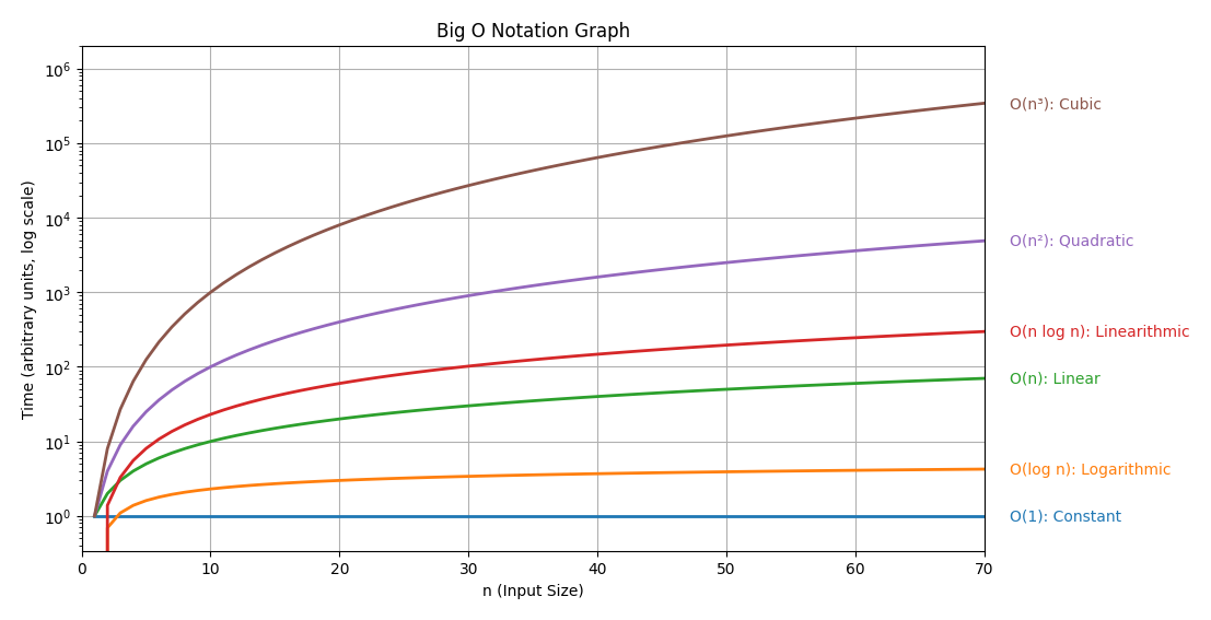
6. Visualizing Growth Rates

Imagine a graph where the x-axis is the input size and the y-axis is the time taken:

O(1) is a flat line.
O(n) is a straight, upward-sloping line.
O(n²) starts off similar for small inputs but grows much faster as n increases.

7. Combining big-o

When you have different parts of an algorithm with their own complexities, combining them depends on whether they run sequentially or are nested within each other.

1. Sequential Operations

If you perform one operation after the other, you add their complexities. For example, if one part of your code is O(n) and another is O(n²), then the total time is:

O(n) + O(n²) = O(n²)

This is because, as n grows, the O(n²) term dominates and the lower-order O(n) becomes negligible.

def sequential_example(nums):
    # First part: O(n)
    for num in nums:
        print(num)

    # Second part: O(n²)
    for i in range(len(nums)):
        for j in range(len(nums)):
            print(nums[i], nums[j])

Here, the overall time complexity is O(n) + O(n²), which simplifies to O(n²).

2. Nested Operations

If one operation is inside another (nested loops), you multiply their complexities. For example, if you have an outer loop that runs O(n) times and an inner loop that runs O(n) times for each iteration, then the total time is:

def nested_example(nums):
    for i in range(len(nums)):          # O(n)
        for j in range(len(nums)):      # O(n) for each i
            print(nums[i], nums[j])

3. Combining Different Parts

In real problems, your code might have a mix of sequential and nested parts.

The key idea is:

Add the complexities for sequential parts.
Multiply the complexities for nested parts.
Drop the lower-order terms and constant factors.

When adding complexities, the dominating term (the one that grows the fastest) is the one that determines the overall Big O notation.

Examples:

def combined_example(arr):
    # Sequential part: Loop that processes each element.
    # This loop runs O(n) times.
    for x in arr:
        print(x)  # O(1) operation per element.

    # Nested part: For each element in arr, loop over arr again.
    # The inner loop is nested within the outer loop, giving O(n) * O(n) = O(n²) operations.
    for x in arr:
        for y in arr:
            print(x, y)  # O(1) operation per inner loop iteration.

# If we call combined_example, the overall complexity is:
# O(n) [from the first loop] + O(n²) [from the nested loops].
# For large n, O(n²) dominates O(n), so we drop the lower-order term and constant factors,
# and the overall time complexity is O(n²).

if __name__ == "__main__":
    sample_list = [1, 2, 3, 4, 5]
    combined_example(sample_list)

# Binary search on a sorted list
def binary_search(arr, target):
    low, high = 0, len(arr) - 1
    while low <= high:
        mid = (low + high) // 2
        if arr[mid] == target:
            return mid
        elif arr[mid] < target:
            low = mid + 1
        else:
            high = mid - 1
    return -1

# Outer loop processes each query, each using binary search
def search_all(sorted_arr, queries):
    results = []
    for query in queries:         # O(n) if queries contains n items
        index = binary_search(sorted_arr, query)  # O(log n)
        results.append(index)
    return results

if __name__ == '__main__':
    # Assume this list is already sorted
    sorted_arr = [1, 2, 3, 4, 5, 6, 7, 8, 9, 10]
    # List of queries (if its size is roughly n, overall complexity is O(n log n))
    queries = [3, 7, 10]
    print("Search results:", search_all(sorted_arr, queries))

Binary Search Function:
This function performs a search on a sorted list in O(log n) time.
Sequential Outer Loop:
The search_all function iterates through each query. For each query, it calls binary search.
- The outer loop contributes O(n) (assuming there are n queries).
- The binary search inside the loop contributes O(log n) per query.
Combined Complexity:
Multiplying the two together gives O(n · log n).
When combined with the rule of dropping lower-order terms and constants, the overall time complexity is O(n log n).

This example demonstrates how nested operations (a loop with an inner binary search) yield an O(n log n) algorithm.

Special Note: If using python sort method, it uses TimSort which worse case is O(n log n)