Coding Interview Patterns
- Getting Started
- Big O
- Brute Force
- Hashmap
- Cycle Sort
- Two Pointers
- Sliding Window
- Getting Started part2
Getting Started
1] Read (and Reread) Carefully and Understand the Problem
Putting the problem in your own words is a powerful way to solidify your understanding of the problem and show a potential interviewer you know what you’re doing.
- Ask Questions to Clarify Doubt: Seek clarifications if anything is unclear. Don't assume details.
- Provide Example Cases to Confirm: Work through examples manually to understand the expected outcomes.
- Plan Your Approach: Outline a logical plan and identify which DS&A could solve the problem. Break problems to sub problems. Always acknowledge the brute force solution if spotted.
Evaluate Input:
- Is it a single array? Or multiple arrays?
- Are there any constraints on the size of the array?
- Can the array contain
- negative numbers
- floating-point numbers
- ...or other data types?
- Is the array presorted?
- Is the array sequential?
- Can the array elements align with the index if its sequential
- Do they have negative values?
Problem Constraints:
- Are there any time complexity requirements for the solution?
- O(1): operations in-place and cannot use additional memory (variables, arrays, dictionaries)
- Are there any space considerations for the solution?
- O(1) means using Hash maps (dictionary)
Output:
- Is it a single value, an array, or something else?
- Are there any specific requirements or constraints on the output format?
Edge Cases:
- Should the algorithm handle edge cases such as
- empty array?
- arrays with only one element?
- arrays with all identical elements?
- Understand the Problem:
- Read and comprehend the problem statement.
- Clarify Doubts:
- Ask the interviewer for clarification if needed.
- Ask Questions:
- Gather more information about the problem.
- Design a Plan:
- Devise an approach to solve the problem.
- Break Down the Problem:
- Divide the problem into smaller sub problems if necessary.
- Choose the Right Data Structures and Algorithms:
- Select appropriate tools based on problem requirements.
- Write Pseudocode:
- Outline the solution logic without worrying about syntax.
- Code Implementation:
- Write the actual code following best practices.
- Test Your Solution:
- Verify correctness and robustness with test cases.
- Optimize if Necessary:
- Improve time or space complexity if possible.
- Handle Errors and Edge Cases:
- Ensure graceful handling of errors and edge cases.
- Review and Debug:
- Check for errors and bugs, and troubleshoot as needed.
- Communicate Your Thought Process:
- Explain your approach and reasoning to the interviewer.
- Be Flexible and Adaptive:
- Adapt your approach based on feedback or new insights.
- Practice Regularly:
- Improve problem-solving skills through practice and mock interviews.
2. If you forget a builtin method, use 'print(dir())' in interactive terminal
This also works on your own methods as well
print(dir(list))

[ __DUNDER_METHODS__ 'append', 'clear', 'copy', 'count', 'extend', 'index', 'insert', 'pop', 'remove', 'reverse', 'sort']
For more in depth information use help(list), but remember to press 'q' in interactive prompt when you want to end process.
|  append(self, object, /)
 |      Append object to the end of the list.
 |
 |  clear(self, /)
 |      Remove all items from list.
 |
 |  copy(self, /)
 |      Return a shallow copy of the list.
 |
 |  count(self, value, /)
 |      Return number of occurrences of value.
 |
 |  extend(self, iterable, /)
 |      Extend list by appending elements from the iterable.
 |
 |  index(self, value, start=0, stop=9223372036854775807, /)
 |      Return first index of value.
 |
 |      Raises ValueError if the value is not present.
 |
 |  insert(self, index, object, /)
 |      Insert object before index.
 |
 |  pop(self, index=-1, /)
 |      Remove and return item at index (default last).
 |
 |      Raises IndexError if list is empty or index is out of range.
 |
 |  remove(self, value, /)
 |      Remove first occurrence of value.
 |
 |      Raises ValueError if the value is not present.
 |
 |  reverse(self, /)
 |      Reverse *IN PLACE*.
 |
 |  sort(self, /, *, key=None, reverse=False)
 |      Sort the list in ascending order and return None.
 |
 |      The sort is in-place (i.e. the list itself is modified) and stable (i.e. the
 |      order of two equal elements is maintained).
 |
 |      If a key function is given, apply it once to each list item and sort them,
 |      ascending or descending, according to their function values.
 |
 |      The reverse flag can be set to sort in descending order.
Big O
How should we describe the speed of an algorithm? One idea is to just count the total number of
primitive operations it does (read, writes, comparisons) when given an input of size n. For example:
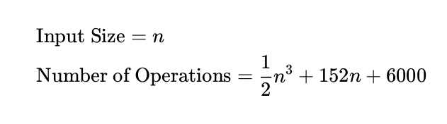
The thing is, it's hard to come up with a formula like this, and the coefficients will vary based on what
processor you use. To simplify this, computer scientists only talk about how the algorithm's speed
scales when n gets very large. The biggest-order term always kills the other terms when n gets very
large (plug in n=1,000,000). So computer scientists only talk about the biggest term, without any
coefficients. The above algorithm has n3 as the biggest term, so we say that:
Time Complexity = O(n3 )
Verbally, you say that the algorithm takes "on the order of n3 operations". In other words, when n gets
very big, we can expect to do around n3 operations.
Computer scientists describe memory based on how it scales too. If your progam needs 51n2 + 200n
units of storage, then computer scientists say Space Complexity = O(n2 ).
Time ≥ Space
The Time Complexity is always greater than or equal to the Space Complexity. If you build a size
10,000 array, that takes at least 10,000 operations. It could take more if you reused space, but it can't
take less - you're not allowed to reuse time (or go back in time) in our universe.
Brute Force
A brute force solution is an approach to problem-solving that involves trying all possible solutions exhaustively, without any optimization or algorithmic insight. In a brute force solution, you typically iterate through all possible combinations or permutations of the input data until you find the solution.
Here are some characteristics of a brute force solution:
While brute force solutions are often simple and conceptually easy to understand, they are generally not suitable for real-world applications or problems with large input sizes due to their inefficiency. Instead, more efficient algorithms and problem-solving techniques, such as dynamic programming, greedy algorithms, or data structures like hashmaps and heaps, are preferred for solving complex problems in a scaleable and efficient manner.
In this brute force solution:
- We iterate over each pair of numbers in the array using two nested loops.
- For each pair of numbers, we calculate their product.
- We keep track of the maximum product found so far.
- Finally, we return the maximum product found after iterating through all pairs of numbers.
While this brute force solution is simple and easy to understand, it has a time complexity of O(n^2) due to the nested loops, where n is the size of the input array. As a result, it may not be efficient for large arrays.
def max_product_bruteforce(nums):
    max_product = float('-inf')
    for i in range(len(nums)):
        for j in range(i + 1, len(nums)):
            product = nums[i] * nums[j]
            max_product = max(max_product, product)
    return max_product

# Example usage:
nums = [3, 5, 2, 6, 8, 1]
result = max_product_bruteforce(nums)
print("Maximum product of two numbers in the array:", result)  # Output: 48 (8 * 6)
A more efficient solution to the problem of finding the maximum product of two numbers in an array can be achieved by using a greedy approach. Here's how it works:
- We can sort the array in non-decreasing order.
- The maximum product of two numbers will either be the product of the two largest numbers (if both are positive) or the product of the largest positive number and the smallest negative number (if the array contains negative numbers).
Here's the implementation of the optimized solution:
def max_product(nums):
    nums.sort()
    n = len(nums)
    # Maximum product will be either the product of the two largest numbers or the product of the largest positive number and the smallest negative number
    return max(nums[-1] * nums[-2], nums[0] * nums[1])

# Example usage:
nums = [3, 5, 2, 6, 8, 1]
result = max_product(nums)
print("Maximum product of two numbers in the array:", result)  # Output: 48 (8 * 6)
This solution has a time complexity of O(n log n) due to the sorting step, which is more efficient than the brute force solution's time complexity of O(n^2). Additionally, it has a space complexity of O(1) since it doesn't require any extra space beyond the input array. Therefore, the optimized solution is more efficient and scalable for larger arrays.
Hashmap
Hashmap Pattern:
- Finding Pairs
- Frequency Counting
- Unique Elements
- Mapping Relationships
- Lookup or Search Operations
- Grouping or Categorization
- Detecting Patterns
- Optimizing Time Complexity
- Avoiding Nested Loops
- Storing State or Metadata
-
Finding Pairs: Problems that involve finding pairs of elements with a specific property, such as pairs that sum up to a target value.
-
Frequency Counting: Problems that require counting the frequency of elements or characters within a collection.
-
Unique Elements: Problems that require ensuring all elements in the collection are unique.
-
Mapping Relationships: Problems that involve mapping relationships between elements, such as mapping an element to its index or another related element.
-
Lookup or Search Operations: Problems that require efficient lookup or search operations based on the properties or values of elements.
-
Grouping or Categorization: Problems that involve grouping or categorizing elements based on certain criteria or properties.
-
Detecting Patterns: Problems that require detecting patterns or similarities between elements or subsets of elements.
-
Optimizing Time Complexity: Problems where using a hashmap can lead to an optimized solution with better time complexity compared to other approaches.
-
Avoiding Nested Loops: Problems where using a hashmap can help avoid nested loops or improve the efficiency of nested loop-based solutions.
-
Storing State or Metadata: Problems that require storing additional state or metadata associated with elements in the collection.
The typically involves a FOR loop and the following components
-
Initialize Hashmap: Create an empty hashmap (dictionary) to store elements and their indices.
-
Iterate Through the List: Use a loop to iterate through each element in the input list
nums. Keep track of the current index using theenumerate()function. -
Calculate Complement: For each element
num, calculate its complement by subtracting it from the target value (target - num). This complement represents the value that, when added tonum, will equal the target. -
Check if Complement Exists: Check if the complement exists in the hashmap. If it does, it means we've found a pair of numbers that sum up to the target. Return the indices of the current element
numand its complement from the hashmap. -
Store Element in Hashmap: If the complement does not exist in the hashmap, it means we haven't encountered the required pair yet. Store the current element
numand its index in the hashmap. This allows us to look up the complement efficiently in future iterations. -
Return Result: If no such pair is found after iterating through the entire list, return an empty list, indicating that no pair of numbers sum up to the target.
def find_pair_with_given_sum(nums, target):
    hashmap = {}  # Create an empty hashmap to store elements and their indices
    for i, num in enumerate(nums):
        complement = target - num  # Calculate the complement for the current element
        if complement in hashmap:
            return [hashmap[complement], i]  # If complement exists in the hashmap, return the indices
        hashmap[num] = i  # Store the current element and its index in the hashmap
    return []  # If no such pair is found, return an empty list

# Example usage:
nums = [2, 7, 11, 15]
target = 9
result = find_pair_with_given_sum(nums, target)
print("Indices of two numbers that sum up to", target, ":", result)  # Output: [0, 1] (2 + 7 = 9)
def high(array):
freq_map = {}
for i in array:
if i in freq_map:
freq_map[i]=freq_map[i] + 1
else:
freq_map[i]=(1)
return freq_map
print(high([5,7,3,7,5,6]))
{5:2 ,7:2, 3:1, 6:1} Cycle Sort
Cycle Sort:
Key Terms
- Missing/Repeated/Duplicate Numbers
- Unsorted Array
- Permutation/Sequence
- In-place Sorting
- Unique Elements
- Indices/Positions
- Range of Numbers
- Fixed Range/Constant Range
- Modifying Indices/Positions
- Array Shuffling
- Swapping Elements
- Array Partitioning
-
Range of Numbers: The problem involves an array containing a permutation of numbers from 1 to N, where N is the length of the array or a known upper bound. The numbers in the array are expected to be consecutive integers starting from 1.
-
Missing Numbers or Duplicates: The problem requires finding missing numbers or duplicates within the given array. Typically, the array may have some missing numbers or duplicates, disrupting the sequence of consecutive integers.
-
No Negative Numbers or Zeroes: The problem specifies that the array contains only positive integers, excluding zero and negative numbers. Cyclic sort works efficiently with positive integers and relies on the absence of zero or negative values.
-
Linear Time Complexity Requirement: The problem constraints or requirements indicate the need for a solution with linear time complexity (O(N)), where N is the size of the array. Cyclic sort achieves linear time complexity as it involves iterating through the array once or a few times.
-
In-Place Sorting Requirement: The problem requires sorting the array in-place without using additional data structures or consuming extra space. Cyclic sort operates by rearranging the elements within the given array, fulfilling the in-place sorting requirement.
Steps
The Cyclic Sort Pattern typically involves a WHILE loop and the following components:
-
Initialization: Start by initializing a pointer
ito 0. -
Iterative Sorting: Repeat the following steps until
ireaches the end of the array:- Look at the elements in the array to calculate the correct index, and see where the range lies. For example [0,5,4,2,1,3] means it is 0-N while [3,4,5,1,2] means its is 1-N.
- 0 to N. the correct index for the number
xat indexiwould bex - 1 to N, the correct index for the number
xat indexiwould bex - 1because index starts at 0, not 1
- 0 to N. the correct index for the number
- Check if the number at index
iis already in its correct position. If it is, incrementito move to the next element. - If the number at index
iis not in its correct position, swap it with the number at its correct index. - Repeat these steps until numbers are placed in their correct positions.
- Look at the elements in the array to calculate the correct index, and see where the range lies. For example [0,5,4,2,1,3] means it is 0-N while [3,4,5,1,2] means its is 1-N.
-
Termination: Once
ireaches the end of the array, the array is sorted. - Once this sorted array is created, typically use another array to cycle through to ensure the index matches with the number
def cyclic_sort(nums):
    i = 0
    while i < len(nums):
        correct_index = nums[i] - 1  # Correct index for the associated number. Since nums is 1-N, then add -1 to prevent error
        if nums[i] != nums[correct_index]:  # If the number is not at its correct index.
            nums[i], nums[correct_index] = nums[correct_index], nums[i]  # Swap the numbers
        else:
            i += 1  # Evaluate the next number if it's already at the correct index
    return nums
# Example usage:
arr = [3, 1, 5, 4, 2]
print(cyclic_sort(arr))

# Ex. of swaps in the Loop
# [5,1,3,4,2]
# [2,1,3,4,5]
# Output: [1, 2, 3, 4, 5]
Visualization:
[4,2,5,6,3,1,7,8]
[6,2,5,4,3,1,7,8]
[1,2,5,4,3,6,7,8]
next iteration [1,2,5,4,3,6,7,8]
next iteration [1,2,5,4,3,6,7,8]
[1,2,3,4,5,6,7,8]
next iteration [1,2,3,4,5,6,7,8]
next iteration [1,2,3,4,5,6,7,8]
next iteration [1,2,3,4,5,6,7,8]
next iteration [1,2,3,4,5,6,7,8]
next iteration [1,2,3,4,5,6,7,8]
next iteration [1,2,3,4,5,6,7,8]

https://youtu.be/jTN7vLqzigc?si=hPJ9mLPanY_d3RTp&t=37
Big O Complexity:
Time: O(n2) but analyze why this works better over time than other SORTING algorithms
Space: O(1) since it is in-place
One of the advantages of cycle sort is that it has a low memory footprint, as it sorts the array in-place and does not require additional memory for temporary variables or buffers. However, it can be slow in certain situations, particularly when the input array has a large range of values. Nonetheless, cycle sort remains a useful sorting algorithm in certain contexts, such as when sorting small arrays with limited value ranges.
Cycle sort is an in-place sorting Algorithm, unstable sorting algorithm, and a comparison sort that is theoretically optimal in terms of the total number of writes to the original array.
- It is optimal in terms of the number of memory writes. It minimizes the number of memory writes to sort (Each value is either written zero times if it’s already in its correct position or written one time to its correct position.)
Two Pointers
Two Pointers:
- Sorted Array/Array is Sorted
- Two Indices/Pointers
- Pointer Manipulation
- Searching/Comparing/Pair Sum
- Closest/Difference
- Intersection/Union of Arrays
- Partitioning/Subarray with Specific Property
- Sliding Window Technique Mentioned Indirectly
- Multiple Pointers Technique
- Removing Duplicates
- Rearranging Array/Reversing Subarray
- Array Traversal
-
Sorted Arrays or Linked Lists: If the problem involves a sorted array or linked list, the Two Pointers Pattern is often applicable. By using two pointers that start from different ends of the array or list and move inward, you can efficiently search for a target element, find pairs with a given sum, or remove duplicates.
-
Window or Range Operations: If the problem requires performing operations within a specific window or range of elements in the array or list, the Two Pointers Pattern can be useful. By adjusting the positions of two pointers, you can control the size and position of the window and efficiently process the elements within it.
-
Checking Palindromes or Subsequences: If the problem involves checking for palindromes or subsequences within the array or list, the Two Pointers Pattern provides a systematic approach. By using two pointers that move toward each other or in opposite directions, you can compare elements symmetrically and determine whether a palindrome or subsequence exists.
-
Partitioning or Segregation: If the problem requires partitioning or segregating elements in the array or list based on a specific criterion (e.g., odd and even numbers, positive and negative numbers), the Two Pointers Pattern is often effective. By using two pointers to swap elements or adjust their positions, you can efficiently partition the elements according to the criterion.
-
Meeting in the Middle: If the problem involves finding a solution by converging two pointers from different ends of the array or list, the Two Pointers Pattern is well-suited. By moving the pointers toward each other and applying certain conditions or criteria, you can identify a solution or optimize the search process.
The Two Pointers Pattern typically involves a WHILE loop and the following components:
-
Initialization: Initialize two pointers (or indices) to start from different positions within the array or list. These pointers may initially point to the beginning, end, or any other suitable positions based on the problem requirements.
-
Pointer Movement: Move the pointers simultaneously through the array or list, typically in a specific direction (e.g., toward each other, in the same direction, with a fixed interval). The movement of the pointers may depend on certain conditions or criteria within the problem.
-
Condition Check: At each step or iteration, check a condition involving the elements pointed to by the two pointers. This condition may involve comparing values, checking for certain patterns, or performing other operations based on the problem requirements.
-
Pointer Adjustment: Based on the condition check, adjust the positions of the pointers as necessary. This adjustment may involve moving both pointers forward, moving only one pointer, or changing the direction or speed of pointer movement based on the problem logic.
-
Termination: Continue moving the pointers and performing condition checks until a specific termination condition is met. This condition may involve reaching the end of the array or list, satisfying a specific criterion, or finding a solution to the problem.
def two_sum(nums, target):
    left, right = 0, len(nums) - 1  # Initialize two pointers at the beginning and end of the array
    while left < right:
        current_sum = nums[left] + nums[right]
        if current_sum == target:
            return [left, right]  # Return the indices of the two numbers that sum up to the target
        elif current_sum < target:
            left += 1  # Move the left pointer to the right to increase the sum
        else:
            right -= 1  # Move the right pointer to the left to decrease the sum
    return []  # If no such pair is found, return an empty list

# Example usage:
nums = [-2, 1, 2, 4, 7, 11]
target = 13
result = two_sum(nums, target)
print("Indices of two numbers that sum up to", target, ":", result)  # Output: [2, 4] (2 + 11 = 13)
Sliding Window
Key terms:
- Fixed Size Subarray
- Maximum/Minimum Subarray
- Consecutive/Continuous Elements
- Longest/Shortest Substring
- Optimal Window
- Substring/Window/Range
- Frequency Count
- Non-overlapping/Subsequence
- Sum/Product/Average in a Window
- Smallest/Largest Window
- Continuous Increasing/Decreasing
-
Finding Subarrays or Substrings: If the problem involves finding a contiguous subarray or substring that meets specific criteria (such as having a certain sum, length, or containing certain elements), the Sliding Window Pattern is likely applicable. Examples include problems like finding the maximum sum subarray, the longest substring with K distinct characters, or the smallest subarray with a sum greater than a target value.
-
Optimizing Brute-Force Solutions: If you have a brute-force solution that involves iterating over all possible subarrays or substrings, the Sliding Window Pattern can often help optimize the solution by reducing unnecessary iterations. By maintaining a window of elements or characters and adjusting its size dynamically, you can avoid redundant computations and achieve better time complexity.
-
Tracking Multiple Pointers or Indices: If the problem involves maintaining multiple pointers or indices within the array or string, the Sliding Window Pattern provides a systematic approach to track and update these pointers efficiently. This is especially useful for problems involving two pointers moving inward from different ends of the array or string.
-
Window Size Constraints: If the problem imposes constraints on the size of the window (e.g., fixed-size window, window with a maximum or minimum size), the Sliding Window Pattern is well-suited for handling such scenarios. You can adjust the window size dynamically while processing the elements or characters within the array or string.
-
Time Complexity Optimization: If the problem requires optimizing time complexity while processing elements or characters in the array or string, the Sliding Window Pattern offers a strategy to achieve linear or near-linear time complexity. By efficiently traversing the array or string with a sliding window, you can often achieve better time complexity compared to naive approaches.
The Sliding Window Pattern typically involves a FOR loop and the following components:
-
Initialization: Start by initializing two pointers or indices: one for the start of the window (left pointer) and one for the end of the window (right pointer). These pointers define the current window.
-
Expanding the Window: Initially, the window may start with a size of 1 or 0. Move the right pointer to expand the window by including more elements or characters from the array or string. The window grows until it satisfies a specific condition or constraint.
-
Contracting the Window: Once the window satisfies the condition or constraint, move the left pointer to contract the window by excluding elements or characters from the beginning of the window. Continue moving the left pointer until the window no longer satisfies the condition or constraint.
-
Updating Results: At each step, update the result or perform necessary operations based on the elements or characters within the current window. This may involve calculating the maximum/minimum value, computing a sum, checking for a pattern, or solving a specific subproblem.
-
Termination: Continue moving the window until the right pointer reaches the end of the array or string. At this point, the algorithm terminates, and you obtain the final result based on the operations performed during each iteration of the window.
def max_sum_subarray(array, k):
    window_sum = 0
    max_sum = float('-inf') #infinitely small number
    window_start = 0

    for window_end in range(len(array)):
        window_sum = window_sum + array[window_end]  # Add the next element to the window

        # If the window size exceeds 'k', slide the window by one element
        if window_end >= k - 1:
            max_sum = max(max_sum, window_sum)  # Update the maximum sum
            print(max_sum)
            window_sum = window_sum - array[window_start]  # Subtract the element going out of the window
            window_start = window_start + 1  # Slide the window to the right
    return max_sum

# Example usage:
array = [1, 3, -1, -3, 5, 3, 6, 7]
k = 3
result = max_sum_subarray(array, k)
print(array)
print("Maximum sum of subarray of size", k, ":", result)  # Output: 16 (subarray: [3, 6, 7])
Getting Started part2
1. Make a good self introduction at the start of the interview
- ✅ Introduce yourself in a few sentences under a minute or 2.
Follow our guide on how to make a good self introduction for software engineers
- ✅ Sound enthusiastic!
Speak with a smile and you will naturally sound more engaging.
- ❌ Do not spend too long on your self introduction as you will have less time left to code.
2. Upon receiving the question, make clarifications
Do not jump into coding right away. Coding questions tend to be vague and underspecified on purpose to allow the interviewer to gauge the candidate's attention to detail and carefulness. Ask at least 2-3 clarifying questions.
- ✅ Paraphrase and repeat the question back at the interviewer.
Make sure you understand exactly what they are asking.
- ✅ Clarify assumptions (Refer to algorithms cheatsheets for common assumptions)
-
A tree-like diagram could very well be a graph that allows for cycles and a naive recursive solution would not work. Clarify if the given diagram is a tree or a graph.
-
Can you modify the original array / graph / data structure in any way?
-
How is the input stored?
-
If you are given a dictionary of words, is it a list of strings or a Trie?
-
Is the input array sorted? (e.g. for deciding between binary / linear search)
-
- ✅ Clarify input value range.
Inputs: how big and what is the range?
- ✅ Clarify input value format
Values: Negative? Floating points? Empty? Null? Duplicates? Extremely large?
- ✅ Work through a simplified example to ensure you understood the question.
E.g., you are asked to write a palindrome checker, before coding, come up with simple test cases like "KAYAK" => true, "MOUSE" => false, then check with the interviewer if those example cases are in line with their expectations
- ❌ Do not jump into coding right away or before the interviewer gives you the green light to do so.
3. Work out and optimize your approach with the interviewer
The worst thing you can do next is jump straight to coding - interviewers expect there to be some time for a 2-way discussion on the correct approach to take for the question, including analysis of the time and space complexity.
This discussion can range from a few minutes to up to 5-10 minutes depending on the complexity of the question. This also gives interviewers a chance to provide you with hints to guide you towards an acceptable solution.
-
✅ If you get stuck on the approach or optimization, use this structured way to jog your memory / find a good approach
-
✅ Explain a few approaches that you could take at a high level (don't go too much into implementation details). Discuss the tradeoffs of each approach with your interviewer as if the interviewer was your coworker and you all are collaborating on a problem.
For algorithmic questions, space/time is a common tradeoff. Let's take the famous Two Sum question for example. There are two common solutions
- Use nested for loops. This would be O(n2) in terms of time complexity and O(1) in terms of space.
- In one pass of the array, you would hash a value to its index into a hash table. For subsequent values, look up the hash table to see if you can find an existing value that can sum up to the target. This approach is O(N) in terms of both time and space. Discuss both solutions, mention the tradeoffs and conclude on which solution is better (typically the one with lower time complexity)
-
✅ State and explain the time and space complexity of your proposed approach(es).
Mention the Big O complexity for time and explain why (e.g O(n2) for time because there are nested for loops, O(n) for space because an extra array is created). Master all the time and space complexity using the algorithm optimization techniques.
-
✅ Agree on the most ideal approach and optimize it. Identify repeated/duplicated/overlapping computations and reduce them via caching. Refer to the page on optimizing your solution.
-
❌ Do not jump into coding right away or before the interviewer gives you the green light to do so.
-
❌ Do not ignore any piece of information given.
-
❌ Do not appear unsure about your approach or analysis.
4. Code out your solution while talking through it
- ✅ Only start coding after you have explained your approach and the interviewer has given you the green light.
- ✅ Explain what you are trying to achieve as you are coding / writing. Compare different coding approaches where relevant.
In so doing, demonstrate mastery of your chosen programming language.
- ✅ Code / write at a reasonable speed so you can talk through it - but not too slow.
You want to type slow enough so you can explain the code, but not too slow as you may run out of time to answer all questions
- ✅ Write actual compilable, working code where possible, not pseudocode.
- ✅ Write clean, straightforward and neat code with as few syntax errors / bugs as possible.
Always go for a clean, straightforward implementation than a complex, messy one. Ensure you adopt a neat coding style and good coding practices as per language paradigms and constructs. Syntax errors and bugs should be avoided as much as possible.
- ✅ Use variable names that explain your code.
Good variable names are important because you need to explain your code to the interviewer. It's better to use long variable names that explain themselves. Let's say you need to find the multiples of 3 in an array of numbers. Name your results array
multiplesOfThreeinstead of array/numbers. - ✅ Ask for permission to use trivial functions without having to implement them.
E.g.
reduce,filter,min,maxshould all be ok to use - ✅ Write in a modular fashion, going from higher-level functions and breaking them down into smaller helper functions.
Let's say you're asked to build a car. You can just write a few high level functions first:
gatherMaterials(),assemble(). Then break downassemble()into smaller functions,makeEngine(),polishWheels(),constructCarFrame(). You could even ask the interviewer if it's ok to not code out some trivial helper functions. - ✅ If you are cutting corners in your code, state that out loud to your interviewer and say what you would do in a non-interview setting (no time constraints).
E.g., "Under non-interview settings, I would write a regex to parse this string rather than using
split()which may not cover certain edge cases." - ✅ [Onsite / Whiteboarding] Practice whiteboard space management
- ❌ Do not interrupt your interviewer when they are talking. Usually if they speak, they are trying to give you hints or steer you in the right direction.
- ❌ Do not spend too much time writing comments.
- ❌ Do not repeat yourself
- ❌ Do not use bad variable names.
- Do not use extremely verbose or single-character variable names, (unless they're common like
i,n) variable names
- Do not use extremely verbose or single-character variable names, (unless they're common like
- ❌ Do not copy and paste code without checking (e.g. some variables might need to be renamed after pasting).
5. After coding, check your code and add test cases
Once you are done coding, do not announce that you are done. Interviewers expect you to start scanning for mistakes and adding test cases to improve on your code.
- ✅ Scan through your code for mistakes - such as off-by-one errors.
Read through your code with a fresh pair of eyes - as if it's your first time seeing a piece of code written by someone else - and talk through your process of finding mistakes
- ✅ Brainstorm edge cases with the interviewer and add additional test cases. (Refer to algorithms cheatsheets for common corner cases)
Given test cases are usually simple by design. Brainstorm on possible edge cases such as large sized inputs, empty sets, single item sets, negative numbers.
- ✅ Step through your code with those test cases.
- ✅ Look out for places where you can refactor.
- ✅ Reiterate the time and space complexity of your code.
This allows you to remind yourself to spot issues within your code that could deviate from the original time and space complexity.
- ✅ Explain trade-offs and how the code / approach can be improved if given more time.
- ❌ Do not immediately announce that you are done coding. Do the above first!
- ❌ Do not argue with the interviewer. They may be wrong but that is very unlikely given that they are familiar with the question.
6. At the end of the interview, leave a good impression
- ✅ Ask good final questions that are tailored to the company.
Read tips and sample final questions to ask.
- ✅ Thank the interviewer
- ❌ Do not end the interview without asking any questions.