00_Getting Started
Template
dsa
m
.
def solve_problem(inputs):
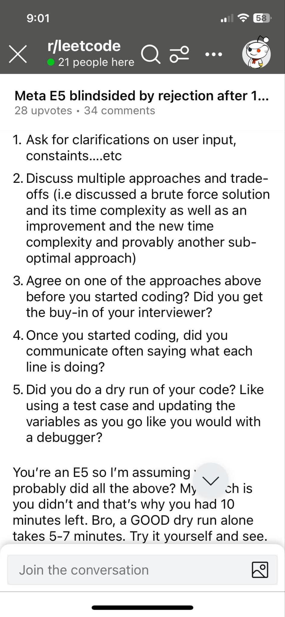
# Step 1: Understand the Problem
# - Parse inputs and outputs.
# - Clarify constraints (e.g., time, space).
# - Identify edge cases.
# Step 2: Plan and Design
# - Think about the brute-force approach.
# - Optimize: Can you use dynamic programming, divide & conquer, etc.?
# - Choose the appropriate data structures (e.g., arrays, hashmaps, heaps).
# Step 3: Implement the Solution
# - Use helper functions for modularity.
# - Write clear, well-commented code.
def helper_function(args):
# Optional: For recursion, BFS, DFS, etc.
pass
# Main logic
result = None # Initialize result or output variable.
# Example logic
# for num in inputs:
# result += num # Or other computations.
return result
# Driver code (for testing locally)
if __name__ == "__main__":
inputs = [] # Replace with example test cases.
print(solve_problem(inputs))Understanding BIG O Calculations
Big O notation is a way to describe how the algorithm grow as the input size increases. Two things it considers:
- Runtime
- Space
1. Basic Idea
-
What It Measures:
Big O notation focuses on the worst-case scenario of an algorithm’s performance. It tells you how the running time (or space) increases as the size of the input grows.-
Guarantee of Performance:
Worst-case analysis provides a guarantee that the algorithm won't perform worse than a certain bound, regardless of the input. -
Adversarial Inputs:
In interviews, interviewers often assume inputs that force the algorithm to perform at its worst, so understanding the worst-case behavior is crucial. -
Comparing Algorithms:
Worst-case complexity gives a clear basis for comparing different algorithms, ensuring that you choose one that performs reliably under all conditions.
-
-
Ignoring Constants:
It abstracts away constants and less significant terms. For instance, if an algorithm takes 3n + 5 steps, it’s considered O(n) because, for large n, the constant 5 and multiplier 3 become negligible compared to n.
2. Common Time Complexities
In order of least dominating term O(1) to most dominating term (the one that grows the fastest)
-
O(1) – Constant Time:
The runtime does not change with the size of the input.-
Example: Accessing an element in a list by its index.
-
-
O(log n) – Logarithmic Time:
The runtime increases slowly as the input size increases.-
Example: Binary search in a sorted list.
-
-
O(n) – Linear Time:
The runtime increases linearly with the input size.-
Example: Iterating through all elements of an array to find a specific value.
-
-
O(n log n):
Often seen in efficient sorting algorithms like mergesort or heapsort.- Example: Sort the list in O(n), then use a Binary search in a sorted list O(logn).
-
O(n²) – Quadratic Time:
The runtime increases quadratically as the input size increases.-
Example: Using two nested loops to compare all pairs in an array.
-
3. Understanding Through Examples
Constant Time – O(1)
def get_first_element(lst):
    return lst[0]
Regardless of list size, only one operation is performed.
Linear Time – O(n)
def find_max(lst):
    max_val = lst[0]
    for num in lst:
        if num > max_val:
            max_val = num
    return max_val
In the find_max function, every element is inspected once, so the time grows linearly with the list size.
Quadratic Time – O(n²)
def print_all_pairs(lst):
    for i in range(len(lst)):
        for j in range(len(lst)):
            print(lst[i], lst[j])
Here, for each element, you’re iterating over the entire list, leading to a quadratic number of comparisons.
4. Why Big O Matters
-
Performance Insight:
Understanding Big O helps you predict how your solution will scale.-
O(n) solution will generally perform better than an O(n²) solution as the input size increases.
-
-
Algorithm Choice:
It allows you to compare different algorithms and select the most efficient one for your needs.-
Discussing Big O can show your understanding of algorithm efficiency.
-
5. Space Complexity
-
Just as you can analyze time complexity, Big O also helps you understand how much memory an algorithm requires relative to the input size.
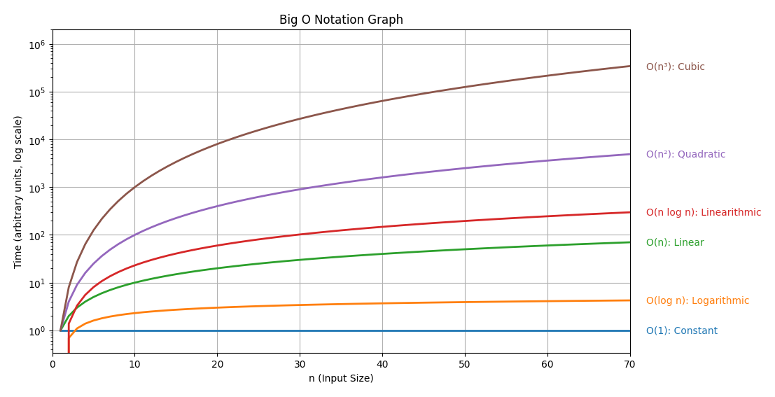
6. Visualizing Growth Rates
Imagine a graph where the x-axis is the input size and the y-axis is the time taken:
-
O(1) is a flat line.
-
O(n) is a straight, upward-sloping line.
-
O(n²) starts off similar for small inputs but grows much faster as n increases.
7. Combining big-o
When you have different parts of an algorithm with their own complexities, combining them depends on whether they run sequentially or are nested within each other.
1. Sequential Operations
If you perform one operation after the other, you add their complexities. For example, if one part of your code is O(n) and another is O(n²), then the total time is:
-
O(n) + O(n²) = O(n²)
This is because, as n grows, the O(n²) term dominates and the lower-order O(n) becomes negligible.
def sequential_example(nums):
    # First part: O(n)
    for num in nums:
        print(num)

    # Second part: O(n²)
    for i in range(len(nums)):
        for j in range(len(nums)):
            print(nums[i], nums[j])
Here, the overall time complexity is O(n) + O(n²), which simplifies to O(n²).
2. Nested Operations
If one operation is inside another (nested loops), you multiply their complexities. For example, if you have an outer loop that runs O(n) times and an inner loop that runs O(n) times for each iteration, then the total time is:
def nested_example(nums):
    for i in range(len(nums)):          # O(n)
        for j in range(len(nums)):      # O(n) for each i
print(nums[i], nums[j])3. Combining Different Parts
In real problems, your code might have a mix of sequential and nested parts.
The key idea is:
-
Add the complexities for sequential parts.
-
Multiply the complexities for nested parts.
-
Drop the lower-order terms and constant factors.
When adding complexities, the dominating term (the one that grows the fastest) is the one that determines the overall Big O notation.
Examples:
def combined_example(arr):
    # Sequential part: Loop that processes each element.
    # This loop runs O(n) times.
    for x in arr:
        print(x)  # O(1) operation per element.

    # Nested part: For each element in arr, loop over arr again.
    # The inner loop is nested within the outer loop, giving O(n) * O(n) = O(n²) operations.
    for x in arr:
        for y in arr:
            print(x, y)  # O(1) operation per inner loop iteration.

# If we call combined_example, the overall complexity is:
# O(n) [from the first loop] + O(n²) [from the nested loops].
# For large n, O(n²) dominates O(n), so we drop the lower-order term and constant factors,
# and the overall time complexity is O(n²).

if __name__ == "__main__":
    sample_list = [1, 2, 3, 4, 5]
    combined_example(sample_list)
# Binary search on a sorted list
def binary_search(arr, target):
low, high = 0, len(arr) - 1
while low <= high:
mid = (low + high) // 2
if arr[mid] == target:
return mid
elif arr[mid] < target:
low = mid + 1
else:
high = mid - 1
return -1
# Outer loop processes each query, each using binary search
def search_all(sorted_arr, queries):
results = []
for query in queries: # O(n) if queries contains n items
index = binary_search(sorted_arr, query) # O(log n)
results.append(index)
return results
if __name__ == '__main__':
# Assume this list is already sorted
sorted_arr = [1, 2, 3, 4, 5, 6, 7, 8, 9, 10]
# List of queries (if its size is roughly n, overall complexity is O(n log n))
queries = [3, 7, 10]
print("Search results:", search_all(sorted_arr, queries))
- Binary Search Function:
This function performs a search on a sorted list in O(log n) time. -
Sequential Outer Loop:
Thesearch_allfunction iterates through each query. For each query, it calls binary search.-
The outer loop contributes O(n) (assuming there are n queries).
-
The binary search inside the loop contributes O(log n) per query.
-
-
Combined Complexity:
Multiplying the two together gives O(n · log n).
When combined with the rule of dropping lower-order terms and constants, the overall time complexity is O(n log n).
This example demonstrates how nested operations (a loop with an inner binary search) yield an O(n log n) algorithm.
Special Note: If using python sort method, it uses TimSort which worse case is O(n log n)
Loops
🟢 Standard
Use when you want to loop directly over the items (values only).
| Input | Example | Output |
|---|---|---|
["apple", "banana"] |
for fruit in ["apple", "banana"]: print(fruit) |
apple banana |
"hi" |
for char in "hi": print(char) |
h i |
{ "a": 1, "b": 2 } |
for key in {"a": 1, "b": 2}: print(key) |
a b |
dict.items() |
for k, v in {"a": 1}.items(): print(k, v) |
a 1 |
🔷 RANGE LOOPS
Use when you need to count, index, or control the steps of iteration.
| Input | Example | Output |
|---|---|---|
range(3) |
for i in range(3): print(i) |
0 1 2 |
range(2, 5) |
for i in range(2, 5): print(i) |
2 3 4 |
range(0, 6, 2) |
for i in range(0, 6, 2): print(i) |
0 2 4 |
range(3, 0, -1) |
for i in range(3, 0, -1): print(i) |
3 2 1 |
range(len(list)) |
for i in range(len(fruits)): print(fruits[i]) |
values in fruits |
🟣 ENUMERATE LOOPS
Use when you want both index and value from a list or iterable.
| Input | Example | Output |
|---|---|---|
["x", "y"] |
for i, v in enumerate(["x", "y"]): print(i, v) |
0 x 1 y |
["a", "b", "c"] |
for i, letter in enumerate(["a", "b", "c"]): ... |
0 a 1 b 2 c |
🧱 NESTED LOOPS
| Loop Type | Input | Example | Output |
|---|---|---|---|
| 🔷 Range | range(2), range(2) |
for i in range(2): for j in range(2): print(i, j) |
0 0, 0 1, 1 0, 1 1 |
| 🔷 Range | 2D array (matrix) by index |
for i in range(len(matrix)):for j in range(len(matrix[0])): |
Access each matrix[i][j] |
| 🔷 Range | All pairs in list | for i in range(len(nums)):for j in range(i+1, len(nums)): |
Pairs (i, j) |
| 🟣 Enumerate | List of lists (2D grid) | for i, row in enumerate(grid):for j, val in enumerate(row): |
(i, j, val) per cell |
| 🟢 Normal | List of lists (values only) | for row in matrix:for val in row: print(val) |
Each cell value |
| 🟢 Normal | Two arrays (cross product) | for a in ["a", "b"]:for n in ["1", "2"]: print(a, n) |
a 1, a 2, b 1, b 2 |
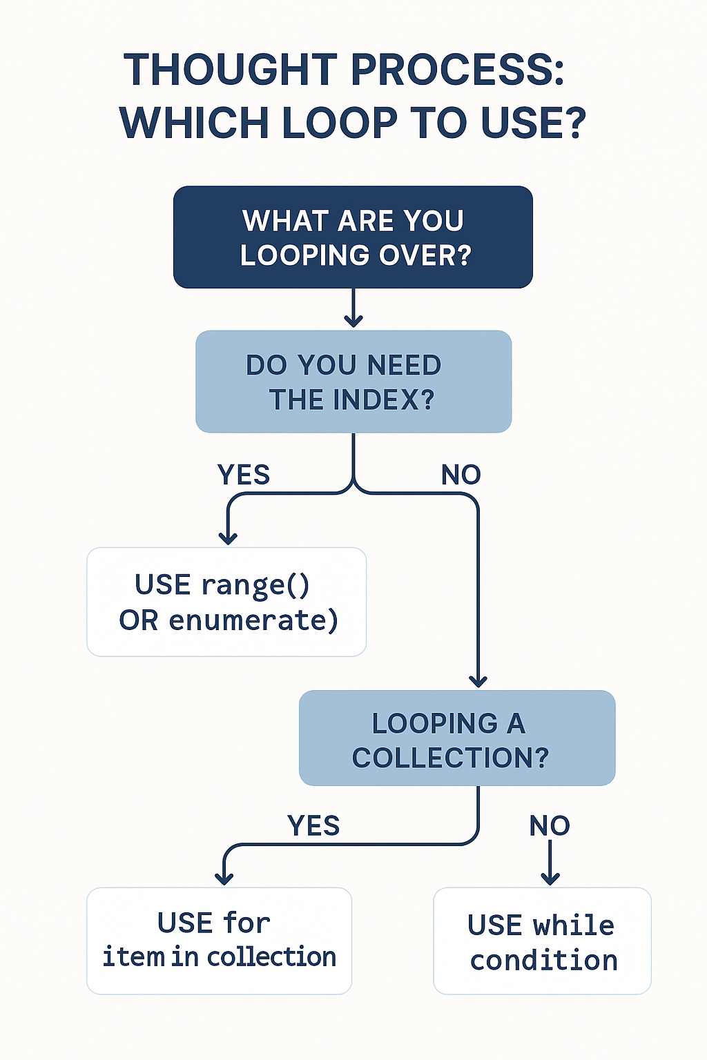
1. ✅ Standard for loop
Use when you want to iterate over items in a list, set, or string.
colors = ['red', 'green', 'blue']
for color in colors:
    print(color)
2. ✅ enumerate() loop
Use when you need both the index and the value.
for i, color in enumerate(colors):
    print(i, color)
3. ✅ range() loop
Use when you want to:
-
Loop a specific number of times
-
Access list items by index
-
Do nested loops
4. ✅ while loop
Use when:
-
You don’t know how many times you’ll loop
-
You’re waiting for a condition to change
x = 0
while x < 5:
    print(x)
    x += 1
📌 Warning: Always make sure the condition will eventually become False or you'll get an infinite loop!
🧠 When to Use Which?
| Loop Type | When to Use |
|---|---|
for item in list |
Clean, readable, item-based loops |
enumerate() |
Index + value |
range() |
Loop by number or index, brute-force logic |
while |
Loop while a condition is true (uncertain end) |
Optional Daily Practice Prompts
Want to write one of each daily?
-
✅
for item in list: print all characters in "hello" -
✅
enumerate(): print index and item of a fruit list -
✅
range(): print numbers 1 to 10 -
✅
while: count down from 5 to 0
Want me to add this to your daily fundamentals checklist or export it as a mini Anki flashcard set or markdown file you can keep open?
OOP for Python
Absolutely! Here's a practical set of Python OOP code examples for each item in your 🧱 Object-Oriented Programming (OOP) checklist — perfect for review or muscle-memory practice.
🧱 Object-Oriented Programming (OOP) in Python — With Code Examples
✅ 1. Create a class with __init__()
class Dog:
    def __init__(self, name):
        self.name = name

d = Dog("Fido")
print(d.name)  # Fido
✅ 2. Add a method to the class
class Dog:
    def __init__(self, name):
        self.name = name

    def bark(self):
        return f"{self.name} says woof!"

d = Dog("Rex")
print(d.bark())  # Rex says woof!
✅ 3. Use @property for a read-only attribute
class Circle:
    def __init__(self, radius):
        self._radius = radius

    @property
    def area(self):
        return 3.14 * self._radius ** 2

c = Circle(3)
print(c.area)  # 28.26
# c.area = 50  # ❌ Error: can't set attribute
✅ 4. Inherit from another class
class Animal:
    def speak(self):
        return "Some sound"

class Dog(Animal):
    def speak(self):
        return "Bark"

d = Dog()
print(d.speak())  # Bark
✅ 5. Override a method
class Animal:
    def speak(self):
        return "Some sound"

class Cat(Animal):
    def speak(self):
        return "Meow"

c = Cat()
print(c.speak())  # Meow
✅ 6. Use super() to call base class method
class Animal:
    def speak(self):
        return "Some sound"

class Dog(Animal):
    def speak(self):
        base = super().speak()
        return base + " + Bark"

d = Dog()
print(d.speak())  # Some sound + Bark
✅ 7. Use __repr__() or __str__()
class Dog:
    def __init__(self, name):
        self.name = name

    def __repr__(self):
        return f"Dog('{self.name}')"

    def __str__(self):
        return f"My dog's name is {self.name}"

d = Dog("Buddy")
print(repr(d))  # Dog('Buddy')
print(str(d))   # My dog's name is Buddy
Absolutely! Here's the full ChatGPT response on polymorphism, polished and formatted so you can save it, review it, or turn it into a markdown or flashcard:
🧱 What is Polymorphism in Python?
🔁 Definition:
Polymorphism means "many forms" — the same function or method behaves differently depending on the object it’s acting on.
💡 Real-World Analogy:
-
You call
draw()on aCircle,Square, orTriangleand each one handles it differently. -
You don’t care how it draws — you just know the object will handle it correctly.
🧪 Python Polymorphism Example 1: Method Overriding
This is classic runtime polymorphism through inheritance:
class Animal:
    def speak(self):
        return "Some sound"

class Dog(Animal):
    def speak(self):
        return "Bark"

class Cat(Animal):
    def speak(self):
        return "Meow"

animals = [Dog(), Cat()]

for animal in animals:
    print(animal.speak())  # Bark, Meow
✅ You call the same method (speak()), but each class handles it differently.
🦆 Python Polymorphism Example 2: Duck Typing
Python doesn’t require a shared parent class — it just cares if the object has the right method.
class Bird:
    def fly(self):
        print("Flapping wings")

class Plane:
    def fly(self):
        print("Engines on")

def lift_off(flier):
    flier.fly()

lift_off(Bird())   # Flapping wings
lift_off(Plane())  # Engines on
✅ As long as the object has a .fly() method, it can be passed in — “if it quacks like a duck...”
🧠 TL;DR:
| Concept | Meaning |
|---|---|
| Polymorphism | Same method name, different behavior |
| Method override | Subclasses implement their own version |
| Duck typing | Type doesn't matter, behavior does |
| Benefit | Cleaner, extensible, decoupled code |
Would you like me to export this explanation as a .md, .txt, or add it to a reference doc for your interview prep?
Data Types
Absolutely — knowing your core data types inside and out is essential for LeetCode and coding interviews. These are the types you’ll see constantly and will use to build efficient solutions.
Here’s a curated list of the must-know data types for LeetCode — including how to use them, when to choose them, and a one-liner to remember what they’re best at.
🧠 LeetCode Data Types You Should Know (Python)
✅ 1. int – Whole numbers
Used for counting, math, binary, etc.
n = 42
🧪 Use cases:
-
Loops, math, binary search, bit manipulation
✅ 2. float – Decimal numbers
Used rarely, but important for precision-sensitive problems.
pi = 3.14
🧪 Watch out for rounding errors.
✅ 3. str – Strings
🔥 High-frequency on LeetCode
s = "leetcode"
🧪 Know:
-
s[::-1]– reverse -
s.split()– split by whitespace -
s.isalnum()– alphanumeric check -
ord(c),chr(n)– ASCII value
✅ 4. list – Ordered, mutable collection
🔥 Most used structure in LeetCode
arr = [1, 2, 3]
🧪 Know:
-
arr.append(x) -
arr.pop(),arr.pop(0) -
arr[::-1] -
arr.sort()vssorted(arr) -
Slicing, binary search, sliding window
✅ 5. tuple – Ordered, immutable collection
Used for keys in sets/dicts or returning multiple values.
t = (1, 2)
🧪 Know:
-
x, y = t -
Useful as hashable keys:
visited[(x, y)] = True
✅ 6. set – Unordered, unique items
🔑 Great for fast lookup and duplicates
s = set([1, 2, 3])
🧪 Know:
-
x in s→ O(1) -
set(list)removes duplicates -
Set operations:
union,intersection,difference
✅ 7. dict – Key-value pairs
🔥 Critical for hash maps / fast lookups
d = {"a": 1, "b": 2}
🧪 Know:
-
d.get(k, default) -
defaultdict(list) -
Frequency count:
Counter(s) -
Keys/values/items iteration
✅ 8. collections.deque – Double-ended queue
⚡ Fast append and popleft() → great for BFS
from collections import deque
q = deque([1, 2])
q.append(3)
q.popleft()
✅ 9. heapq / Min Heap (via list)
💡 Use for priority queue, top K elements
import heapq
h = [5, 3, 8]
heapq.heapify(h)
heapq.heappop(h)
🧪 Python only has min-heaps — invert values for max-heap.
✅ 10. collections.Counter – Fast frequency counting
from collections import Counter
c = Counter("aabbcc")
🧪 Useful for:
-
Anagram check
-
Majority element
-
Multiset behavior
🧠 TL;DR: Memorize These for LeetCode
| Type | What it's good for |
|---|---|
int |
Counting, math |
float |
Precision, rarely needed |
str |
Manipulation, parsing, search |
list |
Arrays, stacks, sliding window |
tuple |
Hashable keys, return multiple items |
set |
Uniqueness, fast lookup |
dict |
Key-value, counting, hash maps |
deque |
BFS, queue (O(1) pops) |
heapq |
Priority queue, top K problems |
Counter |
Fast frequency counting |
Would you like:
-
Anki cards for this?
-
Daily drills where you implement key operations from memory?
-
A printable reference sheet or PDF?